Masters Project - Reproducing Cui Xiang-Han et. al (2020)‘s ’Fast radio bursts: do repeaters and non-repeaters originate in statistically similar ensembles?’

Note

📌 Goal: This notebook tries to reproduce the results from https://ui.adsabs.harvard.edu/abs/2021MNRAS.500.3275C/abstract. As stated in the paper, verbatim

We investigate the statistical classifications for the two groups of samples to see if the non-repeating and repeating FRBs have different origins by employing Anderson–Darling (A–D) test and Mann–WhitneyWilcoxon (M–W–W) test

import pandas as pd
import seaborn as sns; sns.set_theme()
import matplotlib.pyplot as plt
import numpy as np
import scipy

0. Getting The Data

0.1 Source

The data underlying said article are available in the references below:

Spitler et al. (2016);
CHIME/FRB Collaboration (2019a);
Kumar et al. (2019);
CHIME/FRB Collaboration (2019b);
Fonseca et al. (2020).

Some data of FRBs are taken from the data base of FRBCAT, available at http://www.frbcat.org/.

0.1.1 Non-Repeaters

However, I have not been able to effectively filter out repeater from the whole population in the FRBCAT Database. Therefore, I joined it with FRBSTATS where the repeater population has been listed on its utc column rounded to the nearest second.

Deprecated

So I used the FRBSTATS¹ as a proxy with the described filters:

width <= 35
is not identified as repeater
The FRB is observed between FRBCAT’s minimum dan maximum utc datetime
telescope is also available in the FRBCAT catalogue, except ‘CHIME/FRB’²

Using the described filters, I have been able to obtain 88 data points. It is close to the papers sample of 80 ~ 91³

# Load FRBCAT Catalogue

frbcat = pd.read_csv("../data/raw/external/frbcat_20221227.csv", parse_dates=['utc']).rename(
    columns={
        'rop_sampling_time': 'sampling_time',
        'rop_bandwidth': 'bandwidth_MHz',
        'rop_centre_frequency': 'center_freq_MHz'
        })
frbcat['utc'] = frbcat['utc'].round('S')
frbcat = frbcat[frbcat['rmp_width'] <= 35]
frbcat.info()

<class 'pandas.core.frame.DataFrame'>
Int64Index: 107 entries, 0 to 117
Data columns (total 14 columns):
 #   Column           Non-Null Count  Dtype         
---  ------           --------------  -----         
 0   frb_name         107 non-null    object        
 1   utc              107 non-null    datetime64[ns]
 2   telescope        107 non-null    object        
 3   rop_raj          107 non-null    object        
 4   rop_decj         107 non-null    object        
 5   rop_gl           107 non-null    float64       
 6   rop_gb           107 non-null    float64       
 7   sampling_time    106 non-null    float64       
 8   bandwidth_MHz    107 non-null    float64       
 9   center_freq_MHz  107 non-null    float64       
 10  rmp_dm           107 non-null    float64       
 11  rmp_dm_error     107 non-null    float64       
 12  rmp_width        107 non-null    float64       
 13  rmp_snr          104 non-null    float64       
dtypes: datetime64[ns](1), float64(9), object(4)
memory usage: 12.5+ KB

# Load FRBSTATS catalogue and do appropriate filter

# A separate list is used because FRBCAT uses a different name
frbstats_telescope_names_available_in_frbcat = ['Parkes', 'Arecibo', 'Pushchino', 'FAST', 'DSA', 'CHIME', 'WSRT/Apertif', 'UTMOST', 'VLA', 'GBT', 'ASKAP']
frbstats_float_columns = ['l', 'b', 'frequency', 'dm', 'flux', 'width', 'fluence', 'snr', 'redshift']

repeaters_samples = pd.read_csv('../data/raw/external/FRBSTATS2022-11-23_repeaters.csv', index_col=0)
frbstats = pd.read_csv('../data/raw/external/FRBSTATS2022-11-23_population.csv', 
    parse_dates=['utc'], 
    dtype={telescope: float for telescope in frbstats_telescope_names_available_in_frbcat},
    na_values=["-"]
    )
frbstats['utc'].round('S')
# Label repeaters
frbstats["repeater"] = False
frbstats.loc[frbstats["frb"].isin(repeaters_samples["samples"]),"repeater"] = True

# !! Filter is deprecated
# selected_data = frbstats[
#     (frbstats['repeater'] == False) & 
#     (frbstats["width"] <= 35) &
#     (frbstats["telescope"].isin(frbstats_telescope_names_available_in_frbcat)) &
#     (frbstats['telescope'] != 'CHIME') &
#     (frbstats["utc"].between(frbcat["utc"].min(), frbcat["utc"].max()))
#     ]

selected_data = pd.merge(frbcat[['utc', 'sampling_time', 'bandwidth_MHz', 'center_freq_MHz', 'rmp_width']], frbstats[frbstats['repeater'] == False], on='utc')

# Handle NaN values
selected_data.loc[selected_data['width'].isna(), ['width']] = selected_data['rmp_width']
selected_data.loc[selected_data['sampling_time'].isna(), ['sampling_time']] = 0

selected_data.info()

<class 'pandas.core.frame.DataFrame'>
Int64Index: 84 entries, 0 to 83
Data columns (total 25 columns):
 #   Column             Non-Null Count  Dtype         
---  ------             --------------  -----         
 0   utc                84 non-null     datetime64[ns]
 1   sampling_time      84 non-null     float64       
 2   bandwidth_MHz      84 non-null     float64       
 3   center_freq_MHz    84 non-null     float64       
 4   rmp_width          84 non-null     float64       
 5   frb                84 non-null     object        
 6   mjd                84 non-null     float64       
 7   telescope          84 non-null     object        
 8   ra                 84 non-null     object        
 9   dec                84 non-null     object        
 10  l                  84 non-null     float64       
 11  b                  84 non-null     float64       
 12  frequency          84 non-null     float64       
 13  dm                 84 non-null     float64       
 14  flux               77 non-null     float64       
 15  width              84 non-null     float64       
 16  fluence            81 non-null     float64       
 17  snr                82 non-null     float64       
 18  reference          84 non-null     object        
 19  redshift           83 non-null     float64       
 20  redshift_measured  6 non-null      float64       
 21  ra_error           83 non-null     float64       
 22  dec_error          83 non-null     float64       
 23  dm_error           82 non-null     float64       
 24  repeater           84 non-null     bool          
dtypes: bool(1), datetime64[ns](1), float64(18), object(5)
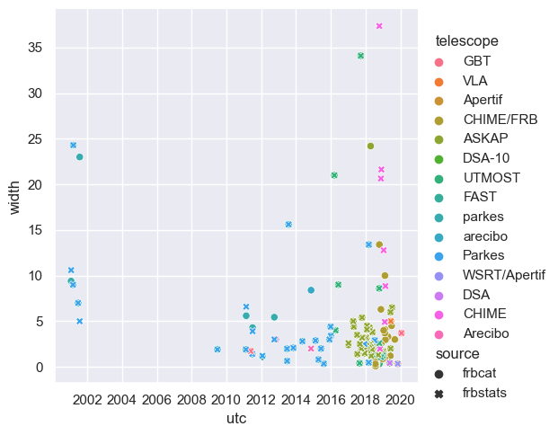
memory usage: 18.5+ KB

In order the accept that both these data describe the same sample, I plotted the overlap between our selected data and the original FRBCAT data.

frbcat_ = frbcat.rename(columns={'frb_name':'frb','rop_raj': 'ra', 'rop_decj': 'dec', 'rop_gb': 'b', 'rop_gl': 'l', 'rmp_width': 'width', 'rmp_dm': 'dm', 'rmp_snr': 'snr'})
frbcat_.loc[:, ['source']] = 'frbcat'
frbstats_ = selected_data[['frb', 'utc', 'telescope', 'ra', 'dec', 'l', 'b', 'dm', 'width', 'snr']]
frbstats_.loc[:, ['source']] = 'frbstats'
frbpopulation_merged = pd.concat([frbcat_, frbstats_])

sns.relplot(data=frbpopulation_merged, x='utc', y='width', style='source', hue='telescope')

<seaborn.axisgrid.FacetGrid at 0x29d3b58f9a0>

0.1.2 Repeaters

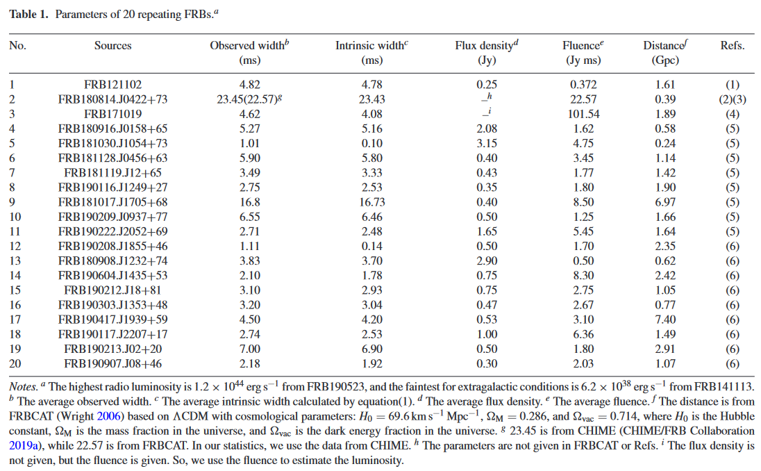
Data on repeaters are easy to obtain. The authors are kind enough to provide table on all 20 samples used in the study.

xianghan = pd.read_csv('../data/raw/external/XiangHan2020_ensemble-repeaters.csv')

	No.	Sources	Observed width (ms)	Intrinsic width (ms)	Flux density (Jy)	Fluence (Jy ms)	Distance (Gpc)	Refs.
0	1	FRB121102	4.82	4.78	0.25	0.372	1.61	(1)
1	2	FRB180814.J0422+73	22.57	23.43	nan	22.57	0.39	(2)(3)
2	3	FRB171019	4.62	4.08	nan	101.54	1.89	(4)
3	4	FRB180916.J0158+65	5.27	5.16	2.08	1.62	0.58	(5)
4	5	FRB181030.J1054+73	1.01	0.1	3.15	4.75	0.24	(5)
5	6	FRB181128.J0456+63	5.9	5.8	0.4	3.45	1.14	(5)
6	7	FRB181119.J12+65	3.49	3.33	0.43	1.77	1.42	(5)
7	8	FRB190116.J1249+27	2.75	2.53	0.35	1.8	1.9	(5)
8	9	FRB181017.J1705+68	16.8	16.73	0.4	8.5	6.97	(5)
9	10	FRB190209.J0937+77	6.55	6.46	0.5	1.25	1.66	(5)
10	11	FRB190222.J2052+69	2.71	2.48	1.65	5.45	1.64	(5)
11	12	FRB190208.J1855+46	1.11	0.14	0.5	1.7	2.35	(6)
12	13	FRB180908.J1232+74	3.83	3.7	2.9	0.5	0.62	(6)
13	14	FRB190604.J1435+53	2.1	1.78	0.75	8.3	2.42	(6)
14	15	FRB190212.J18+81	3.1	2.93	0.75	2.75	1.05	(6)
15	16	FRB190303.J1353+48	3.2	3.04	0.47	2.67	0.77	(6)
16	17	FRB190417.J1939+59	4.5	4.2	0.53	3.1	7.4	(6)
17	18	FRB190117.J2207+17	2.74	2.53	1	6.36	1.49	(6)
18	19	FRB190213.J02+20	7	6.9	0.5	1.8	2.91	(6)
19	20	FRB190907.J08+46	2.18	1.92	0.3	2.03	1.07	(6)

1.0 Preprocessing

1.1 Parameters

We first process our data to uncover these parameters:

Pulse width
Radio Luminosity

1.1.1 Pulse Width

Since the pulse width in the FRBCAT is the observed width, which is easily affected by dispersion, to study the pulse width more accurately, we need to introduce the intrinsic width that is estimated by equation: \[ t_i = \sqrt{t^2_\text{obs} − t^2_\text{DM} − t^2_s} \] In the above formula, \(t_i(t_\text{obs})\) is the intrinsic width (observed width), with \(t_s\) being the sampling time that depends on the instrument, and \(t_\text{DM}\) is the dispersion smearing time-scale as calculated in the following: \[ t_\text{DM} = 8.3 \times 10^{−3} \text{DM}\frac{\Delta ν_\text{MHz}}{ν^3_\text{GHz}} ms, \] where DM is the dispersion measure, \(\Delta ν_\text{MHz}\) is the channel bandwidth in the unit of MHz, and \(ν_\text{GHz}\) is the central frequency in the unit of GHz. Therefore, the pulse width in the following text represents the intrinsic width.

def dispersion_smearing_timescale(dispersion_measure, bandwidth_MHz, center_freq_GHz) -> float:
    return 8.3e-6 * dispersion_measure * (bandwidth_MHz / center_freq_GHz**3)

def instrinsic_width(observed_width, sampling_time, dispersion_measure, bandwidth_MHz, center_freq_GHz) -> float:
    return np.sqrt(abs((observed_width**2 - dispersion_smearing_timescale(dispersion_measure, bandwidth_MHz, center_freq_GHz)**2 - sampling_time**2)))

selected_data.loc[:, 'intrinsic_width_ms'] = instrinsic_width(
    selected_data['width'], 
    selected_data['sampling_time'], 
    selected_data['dm'], 
    selected_data['bandwidth_MHz'], 
    selected_data['center_freq_MHz']*0.001)

frbcat.loc[:, 'intrinsic_width_ms'] = instrinsic_width(
    frbcat['rmp_width'],
    frbcat['sampling_time'],
    frbcat['rmp_dm'],
    frbcat['bandwidth_MHz'],
    frbcat['center_freq_MHz']*0.001
)

1.1.2 Radio Luminosity

Radio luminosity is estimated using the formula below: \[ L_\text{radio} \approx SD^2 \] where \(S\) is the flux density and \(D\) is the luminosity distance

Jy_to_erg_s = 1e-23 # erg s-1 cm-2 Hz-1
Gpc_to_m = 3.0857e16 * 1e6 # m
m_to_cm = 100 #cm

def radio_luminosity_approx(flux_density: float, luminosity_distance: float) -> float:
    """Approximation of radio luminosity

    Args:
        flux_density (float): flux density in Jy
        luminosity_distance (float): Luminosity distance in Gpc

    Returns:
        float: radio luminosity in erg/s /Hz
    """
    flux_density_erg_s = flux_density*Jy_to_erg_s
    luminosity_distance_cm = luminosity_distance*Gpc_to_m*m_to_cm
    return flux_density_erg_s*(luminosity_distance_cm**2)

The formula for luminosity distance in this notebook is taken from the python implementation of

c_km_s = 299792.458 # velocity of light in km/sec
H_0_km_s_Mpc: float = 69.6 # km s^-1 Mpc^-1
def luminosity_distance(z: float, Omega_matter: float = 0.268, Omega_vacuum:float = 0.714, H_0_km_s_Mpc: float = 69.6) -> float:
    """Calculate luminosity distance at redshift based on the python's implementation of [CosmoCalc](https://www.astro.ucla.edu/~wright/CosmoCalc.html)

    Args:
        z (float): redshift
        Omega_matter (float, optional): Total matter density. Defaults to 0.268.
        Omega_vacuum (float, optional): Cosmological Constant. Defaults to 0.714.
        H_0_km_s_Mpc (float, optional): Hubbles constant in km s^-1 Mpc^-1. Defaults to 69.6.

    Returns:
        float: Luminosity distance in Mpc
    """
    h = H_0_km_s_Mpc/100.
    Omega_radiation = 4.165E-5/(h*h)   # includes 3 massless neutrino species, T0 = 2.72528
    Omega_curvature = 1-Omega_matter-Omega_radiation-Omega_vacuum


    z = z[0]
    az = 1.0/(1+1.0*z)
    DTT = 0.0
    DCMR = 0.0
    n=1000         # number of points in integrals
    # do integral over a=1/(1+z) from az to 1 in n steps, midpoint rule
    for i in range(n):
        a = az+(1-az)*(i+0.5)/n
        adot = np.sqrt(Omega_curvature+(Omega_matter/a)+(Omega_radiation/(a*a))+(Omega_vacuum*a*a))
        DTT = DTT + 1./adot
        DCMR = DCMR + 1./(a*adot)

    DTT = (1.-az)*DTT/n
    DCMR = (1.-az)*DCMR/n

    ratio = 1.00
    x = np.sqrt(abs(Omega_curvature))*DCMR
    if x > 0.1:
        if Omega_curvature > 0:
            ratio =  0.5*(np.exp(x)-np.exp(-x))/x 
        else:
            ratio = np.sin(x)/x
    else:
        y = x*x
        if Omega_curvature < 0: y = -y
        ratio = 1. + y/6. + y*y/120.
    DCMT = ratio*DCMR
    DA = az*DCMT
    DL = DA/(az*az)
    DL_Mpc = (c_km_s/H_0_km_s_Mpc)*DL
    return DL_Mpc

def redshift_from_distance(distance):
    return distance*H_0_km_s_Mpc/c_km_s

selected_data['radio_luminosity']   = radio_luminosity_approx(
                                        selected_data['flux'], 
                                        luminosity_distance(z=selected_data['redshift'])*1000
                                    )
xianghan['radio_luminosity']        = radio_luminosity_approx(
                                        xianghan['Flux density (Jy)'], 
                                        luminosity_distance(
                                            z=redshift_from_distance(xianghan['Distance (Gpc)'])
                                        )*1000
                                    )

selected_data['radio_luminosity'].describe()

count    7.700000e+01
mean     1.661798e+39
std      2.601721e+39
min      3.006860e+36
25%      4.780137e+37
50%      5.396929e+38
75%      2.081672e+39
max      1.137210e+40
Name: radio_luminosity, dtype: float64

xianghan['radio_luminosity'].describe()

count    1.800000e+01
mean     2.319993e+32
std      2.213047e+32
min      6.173843e+31
25%      1.006336e+32
50%      1.234769e+32
75%      2.315191e+32
max      7.779042e+32
Name: radio_luminosity, dtype: float64

We can see that the range is not quite the same as stated in the paper:

Repeaters: ∼10³⁹ to ∼10⁴² erg s⁻¹
Non-repeaters: ∼10³⁸ to ∼10⁴⁴ erg s⁻¹

which possibly means that there are parts of the calculations that I am missing.

2.0 Statistical Test

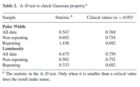
2.1 Anderson–Darling Test

An Anderson–Darling test (A-D test) is used to measure the likelihood that a sample follows a certain distribution.

from scipy.stats import anderson

anderson_width_all = anderson([*xianghan['Intrinsic width (ms)'], *selected_data['intrinsic_width_ms'].dropna()], dist='norm')
anderson_width_xianghan = anderson(xianghan['Intrinsic width (ms)'], dist='norm')
anderson_width_nonrepeater = anderson(selected_data['intrinsic_width_ms'].dropna(), dist='norm')

	Sample	Statistic	Critical values (\(\alpha\) = 0.05)
0	All data	12.9237	0.76
1	Non-repeating	11.0479	0.754
2	Repeating	2.38607	0.692

anderson_lumo_all = anderson([*xianghan['radio_luminosity'].dropna(), *selected_data['radio_luminosity'].dropna()], dist='norm')
anderson_lumo_xianghan = anderson(xianghan['radio_luminosity'].dropna(), dist='norm')
anderson_lumo_nonrepeater = anderson(selected_data['radio_luminosity'].dropna(), dist='norm')

	Sample	Statistic	Critical values (\(\alpha\) = 0.05)
0	All data	13.3245	0.757
1	Non-repeating	9.08615	0.751
2	Repeating	2.24584	0.687

Clearly, the results are different from what is stated from the paper.

Even for the exact same data on the variable xianghan (Repeating) and the exact copy of the Intrinsic width (ms) parameters, the values are different. I have been trying to figure that out for about 3 weeks but no avail. Here are the things that I have tried:

A custom Anderson-Darling function which yielded higher values.
Excluding some values (No. 2, 12, 20) which yielded close enough statistic (1.43080) but I doubt that is the reason.

I decided to stop trying and move on to something else.

Footnotes

https://www.herta-experiment.org/frbstats/↩︎
Even with the described filters, the CHIME/FRB telescope dominates the dataset making up >500 data points while it is not that prominent in FBRCAT and also the total data points is less than 100↩︎
The paper mentioned both numbers. The lower limit of 80 is mentioned in the conclusion but the upper limit of 91 is mentioned in the abstract. So I took it as a range instead.↩︎